Unconditional density estmation

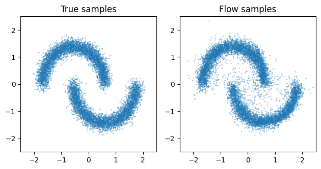
Here we will use a masked_autoregressive_flow with a RationalQuadraticSpline transformer to approximate the “two-moons” distribution. For a list of available flow architectures, please see flowjax.flows.

Importing the required libraries.

import jax.numpy as jnp
import jax.random as jr
import matplotlib.pyplot as plt

from flowjax.bijections import RationalQuadraticSpline
from flowjax.distributions import Normal
from flowjax.flows import masked_autoregressive_flow
from flowjax.tasks import two_moons
from flowjax.train import fit_to_data

Generating the the toy dataset.

n_samples = 10000
rng = jr.key(0)
x = two_moons(rng, n_samples)
x = (x - x.mean(axis=0)) / x.std(axis=0)  # Standardize

We can now create the flow. We use a normal base distribution, and define the spline transformer to have 8 knots on the interval [-4,4]. Note that we could use other bijections for the transformer (e.g. Affine).

key, subkey = jr.split(jr.key(0))
flow = masked_autoregressive_flow(
    subkey,
    base_dist=Normal(jnp.zeros(x.shape[1])),
    transformer=RationalQuadraticSpline(knots=8, interval=4),
)

Training the flow.

key, subkey = jr.split(key)
flow, losses = fit_to_data(subkey, flow, x, learning_rate=1e-3)

 13%|█▎        | 13/100 [00:14<01:37,  1.12s/it, train=1.5686557, val=1.5484393 (Max patience reached)]

We can use the flow to evaluate the density of arbitrary points

five_points = jnp.ones((5, 2))
flow.log_prob(five_points)

Array([-8.574494, -8.574494, -8.574494, -8.574494, -8.574494], dtype=float32)

and we can sample the flow

key, subkey = jr.split(key)
x_samples = flow.sample(subkey, (n_samples,))

fig, axs = plt.subplots(ncols=2)

axs[0].scatter(x[:, 0], x[:, 1], s=0.1)
axs[0].set_title("True samples")

axs[1].scatter(x_samples[:, 0], x_samples[:, 1], s=0.1)
axs[1].set_title("Flow samples")

lims = (-2.5, 2.5)
for ax in axs:
    ax.set_xlim(lims)
    ax.set_ylim(lims)
    ax.set_aspect("equal")

plt.tight_layout()
plt.show()