Variational inference

We will fit a simple 1D Bayesian linear regression with known variance. The likelihood is given by,

\[y \sim \mathcal{N}(w_0 + w_1x,\ 1),\]

and the prior is,

\[w_0, w_1 \sim N(0,\ I).\]

import jax.numpy as jnp
import jax.random as jr
import matplotlib.pyplot as plt
from jax.scipy.stats import multivariate_normal, norm

from flowjax.bijections import Affine
from flowjax.distributions import StandardNormal
from flowjax.flows import masked_autoregressive_flow
from flowjax.train.losses import ElboLoss
from flowjax.train.variational_fit import fit_to_variational_target

# generate observed data
data_key = jr.PRNGKey(0)
w_0 = 0.5
w_1 = -0.5

n = 20
key, x_key, noise_key = jr.split(data_key, 3)
x = jr.uniform(x_key, shape=(n,)) * 4 - 2
y = w_0 + w_1 * x + jr.normal(noise_key, shape=(n,))

We can define our objective, via the unnormalised posterior distribution. This maps samples \(w\) to a vector of unnormalised probabilites

def unormalized_posterior(w):
    likelihood = norm.logpdf(y, w[0] + x * w[1]).sum()
    prior = norm.logpdf(w).sum()  # Standard normal prior
    return (likelihood + prior).sum()

We define and fit the flow. Note that we set invert=False, which loosely speaking specifies that we prioritise faster sample and sample_and_log_prob methods for the flow, instead of a fast log_prob method. The evidence lower bound (ELBO) approximation is computed using the sample_and_log_prob method.

loss = ElboLoss(unormalized_posterior, num_samples=100)

key, flow_key, train_key = jr.split(key, 3)
flow = masked_autoregressive_flow(
    flow_key, base_dist=StandardNormal((2,)), transformer=Affine(), invert=False,
)

# Train the flow variationally
flow, losses = fit_to_variational_target(
    train_key, flow, loss, learning_rate=1e-3, steps=400,
)

100%|██████████| 400/400 [00:02<00:00, 155.93it/s, loss=29.5]

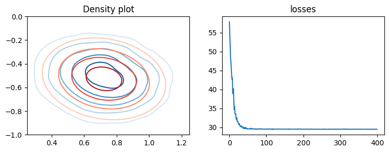
We can now visualise the learned posterior, here using contour plots to show the approximate (blue) and true (red) posterior

def plot_density(
    ax, density_fn, xmin=-5, xmax=5, ymin=-5, ymax=5, n=100, levels=None, cmap="Blues",
):
    xvalues = jnp.linspace(xmin, xmax, n)
    yvalues = jnp.linspace(ymin, ymax, n)
    x, y = jnp.meshgrid(xvalues, yvalues)

    points = jnp.hstack([x.reshape(-1, 1), y.reshape(-1, 1)])

    log_prob = density_fn(points).reshape(n, n)
    prob = jnp.exp(log_prob)

    ax.contour(
        prob, levels=levels, extent=[xmin, xmax, ymin, ymax], origin="lower", cmap=cmap,
    )

    ax.set_xlim(xmin, xmax)
    ax.set_ylim(ymin, ymax)


fig, axes = plt.subplots(ncols=2, figsize=(9, 3))
axes[0].set_title("Density plot")

kwargs = {"xmin": 0.25, "xmax": 1.25, "ymin": -1, "ymax": 0, "levels": 5}
plot_density(axes[0], flow.log_prob, cmap="Blues", **kwargs)

# True posterior for comparison
_x = jnp.vstack([jnp.ones_like(x), x])  # full design matrix
cov = jnp.linalg.inv(_x.dot(_x.T) + jnp.eye(2))
mean = cov.dot(_x).dot(y)


def true_posterior_log_prob(theta):
    return multivariate_normal.logpdf(theta, mean, cov)


plot_density(axes[0], true_posterior_log_prob, cmap="Reds", **kwargs)
axes[1].set_title("losses")
axes[1].plot(losses)

[<matplotlib.lines.Line2D at 0x7eff79b56cd0>]

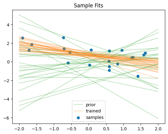
We can visualise the regression fits

x_inspect = jnp.linspace(2, -2, n)
plots = [
    ("prior", StandardNormal((2,)), "tab:green"),
    ("trained", flow, "tab:orange"),
]
n_samples = 25

for label, flow, colour in plots:
    key, sample_key = jr.split(key)
    w = flow.sample(sample_key, (n_samples,))
    for ix, (w_0, w_1) in enumerate(w):
        y_inspect = w_0 + w_1 * x_inspect
        lab = label if ix == 0 else None
        plt.plot(x_inspect, y_inspect, alpha=0.3, c=colour, label=lab)

plt.scatter(x, y, label="samples")
plt.title("Sample Fits")
plt.legend()
plt.show()